ONDAS CINEMÁTICO-DINÁMICAS MIXTAS DESBANCADAS
Profesor Emérito de Ingeniería Civil y Ambiental
Universidad Estatal de San Diego,
California
1. INTRODUCCIÓN
En el modelamiento de ondas de inundación, a menudo la primera pregunta
que se presenta es la siguiente: żQué tipo de onda debo utilizar? Al respecto, observamos
que las ondas cinemáticas y
difusivas están ya bien establecidas en la práctica. Por otro lado, reconocemos que las ondas
dinámicas de Lagrange no se prestan generalmente a aplicaciones de ondas
de inundación.
Durante los últimos cincuenta ańos, el enfoque que parece haber prevalecido en algunos
sectores de la ingeniería hidráulica es el siguiente: "Olvídémosnos de los distintos tipos de ondas; utilicemos la
solución completa de las ecuaciones de St. Venant en todas las aplicaciones y dejemos
que la computadora haga los cálculos". Observamos que la teoría y la práctica
han confirmado que este enfoque es generalmente fútil.
Nuestro objetivo es mostrar que el uso exclusivo de ondas mixtas es,
en el mejor de los casos, inútil, y en el peor, incorrecto, siendo muy probable
que lleve a pérdida de tiempo y recursos. En un esfuerzo por propiciar la claridad,
en la siguiente
sección enumeramos los diferentes tipos de ondas que se utilizan actualmente,
a la vez que detallamos su naturaleza y propiedades.
2. TIPOS DE ONDAS
En el flujo unidimensional no permanente en canales abiertos se utilizan generalmente
los siguientes tipos de ondas: (1) cinemática; (2) difusiva;
(3) mixta; y (4) dinámica. Las ondas cinemáticas excluyen los términos
de inercia y gradiente de presiones; las ondas difusivas excluyen sólo los términos
de inercia; las ondas mixtas no excluyen ningún
término, y las ondas dinámicas excluyen los términos de fricción y gravedad (Tabla 1).
Los términos excluidos se eliminan porque se asume que son demasiado pequeńos
para afectar materialmente las propiedades de la onda en cuestión.
3. PROPIEDADES DE LAS ONDAS
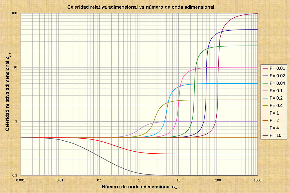
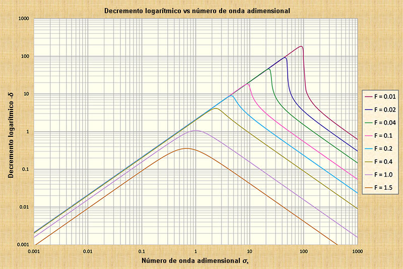
Ponce y Simons (1977) han examinado detalladamente las propiedades de los diversos tipos de ondas (Figs. 2 y 3).
Ellos utilizaron la teoría de la estabilidad lineal para determinar las funciones
de celeridad y atenuación para las siguientes ondas: (1) cinemáticas, (2) difusivas, (3) mixtas, y
Las ondas cinemáticas son las de Seddon (1900), mientras que las ondas dinámicas son las
de Lagrange (1788). Las ondas cinemático-dinámicas mixtas, a las que aquí referimos
simplemente como ondas mixtas, son aquéllas que se encuentran hacia
el centro-derecha del espectro del número de onda adimensional (Fig. 2). Estas ondas aparecieron en los modelos numéricos desarrollados a partir
de la década de 1970 para resolver las ecuaciones completas de St. Venant; véase,
por ejemplo, Fread (1985). Estos modelos han sido ampliamente denominados modelos
de "ondas dinámicas", aunque lo inapropiado del nombre
ha causado confusión con
las ondas dinámicas de Lagrange (1788), establecidas desde hace más de dos siglos.
Las ondas difusivas se encuentran a la derecha de las ondas cinemáticas y a la
izquierda de las ondas mixtas en el espectro del número de onda adimensional
(Fig. 2). A diferencia de las ondas cinemáticas, que presentan difusión cero,
las ondas difusivas tienen una cantidad de difusión pequeńa pero perceptible.
Sin embargo, esta difusión es pequeńa en comparación con la de las ondas mixtas
(Fig. 3). Observamos que la inclusión del término gradiente de presiones (Tabla 1)
es directamente responsable por la difusión.
La Figura 2 muestra que las ondas cinemáticas de Seddon, que se encuentran hacia la izquierda del espectro del número de onda adimensional, presentan una celeridad constante y, por lo tanto, no son difusivas. Siguiendo el mismo razonamiento, las ondas dinámicas de Lagrange, situadas hacia la derecha de la Fig. 2, tampoco son difusivas. Sin embargo, se muestra que las ondas mixtas, que se encuentran hacia el centro-derecha y que muestran una celeridad altamente variable, son fuertemente difusivas. La cantidad de difusión, caracterizada por el decremento logarítmico δ, varía con el número de Froude predominante (Fig. 3) (Wylie, 1966). Una mayor difusión corresponde a números de Froude más bajos, siempre que este último permanezca por debajo del valor umbral F = 2, aplicable para la fricción de Chezy en canales hidráulicamente anchos (Figs. 2 y 3).
4. ONDAS CINEMÁTICAS
De hecho, una onda cinemática puede considerarse como la onda de inundación veritas.
En este momento, parece conveniente citar a
Lighthill y Whitham (1955),
quienes establecieron las bases de la teoría de las ondas cinemáticas. Observaron con atención lo siguiente (op, cit, p. 285):
5. ONDAS DIFUSIVAS
A diferencia de las ondas cinemáticas, las ondas difusivas
están sujetas a una pequeńa cantidad de difusión. Se encuentran
inmediatamente a la derecha de las ondas cinemáticas en el espectro
de números de onda adimensionales, propiamente dentro
del rango 0,01 ≤ σ* ≤ 0,17 (Fig. 2)
Las ondas de inundación típicas se difusionan un tanto;
entonces, las ondas difusivas son un modelo apropiado
de propagación de ondas de inundación. Complementan
muy bien a las ondas cinemáticas, aunque encuentran su
mejor aplicación en los casos en que la difusión de las
ondas es apreciable, forzando la necesidad de su cálculo.
Sin embargo, surge el siguiente problema:
Los modelos numéricos de ondas cinemáticas
convencionales muestran de hecho cierta cantidad de difusión.
La cuestión de cómo manejar mejor la difusión numérica ha
sido resuelta por Cunge (1969), quien propuso una coincidencia
de la difusión numérica del esquema mismo con la difusión física
de la ecuación de la onda cinemática con difusión,
es decir, la ecuación de la onda difusiva. Este desarrollo
llevó al método Muskingum-Cunge de enrutamiento
de inundaciones, una alternativa de base física al
clásico método Muskingum (Ponce, 2014a).
6. ONDAS DINÁMICAS
Las ondas dinámicas clásicas son las de Lagrange (1788). Más recientemente,
Fread (1985) y otros se han referido a las ondas cinemático-dinámicas mixtas como
ondas "dinámicas", mientras que aquí nos referimos a ellas simplemente como
ondas "mixtas". La confusión semántica es realmente desafortunada. En un intento
de contribuir a solucionar este problema, aquí utilizamos el adjetivo "dinámico"
para referirnos únicamente a las ondas de Lagrange.
Las ondas dinámicas presentan una celeridad de onda constante para el
número de onda adimensional σ* ≥ 100 para la mayoría de los números de Froude,
y σ* ≥ 1000 para todos los números de Froude (Fig. 2). Esto significa
de manera concluyente, como en el caso de las ondas cinemáticas, que las
ondas dinámicas de Lagrange no están sujetas a difusión.
Está claro que las ondas dinámicas de Lagrange no son las típicas ondas de inundación.
Su tamańo es demasiado pequeńo para constituir un verdadero riesgo.
Su aplicación se limita a la propagación de ondas cortas en canales de
irrigación y fuerza eléctrica, en los cuales la escala de la perturbación es tal que
típicamente
la onda puede percibirse a simple vista. A diferencia de las ondas de
inundación, que son ondas de masa que presentan una sola onda que
viaja aguas abajo, las ondas dinámicas clásicas son ondas de energía,
que presentan dos ondas que viajan en direcciones opuestas en flujo
subcrítico, y en una sola dirección (aguas abajo) en flujo supercrítico.
A modo de reiteración, nos permitimos aquí hacer un comentario
sobre la verdadera causa de la difusión de las ondas. La difusión se produce por la
interacción del gradiente de presiones con los términos de fricción y
gravedad (Tabla 1, Fila 2). Definida de manera más precisa, la
difusión se produce por la interacción de los términos no cinemáticos (inercia y/o gradiente de presiones), con los términos
cinemáticos (fricción y gravedad) (Tabla 1, Fila 3)
(Ponce, 1982).
La cantidad de difusión es proporcional a la interacción
entre los términos cinemáticos y dinámicos de la ecuación de movimiento.
La falta de términos cinemáticos da como resultado una difusión cero,
representada por las curvas hacia el extremo derecho de la Fig. 2. Por
el contrario, la falta de términos dinámicos también da como resultado
una difusión cero, representada por la curva en el extremo izquierdo de la Fig. 2.
7. ONDAS MIXTAS
En esta sección tratamos el otro tipo de onda que queda:
la onda cinemática-dinámica mixta, para abreviar, la onda "mixta" del flujo
inestable en canales abiertos. Dado que, por definición, esta onda presenta
componentes tanto cinemáticos como dinámicos en cantidades comparables, se concluye que debe ser fuertemente difusiva.
La respuesta a esta pregunta es ˇClaro que sí! De hecho, la onda cinemático-dinámica mixta
es muy fuertemente difusiva. Es más, ˇes la más difusiva de todas las ondas
consideradas en este trabajo! Ante este hecho, la pregunta que persiste es la de si la onda
mixta puede ser interpretada como una onda de inundación o no. Para responder con
precisión, recurrimos una vez más al esclarecedor trabajo de
Ponce y Simons (1977) y a su cálculo analítico de las funciones de celeridad y atenuación
para todo tipo de ondas en aguas poco profundas. Las cantidades de atenuación de las
olas calculadas por Ponce y Simons (ver detalle en el Cuadro A) se representan
en la Fig. 3 y se complementan con la Tabla 2.
Dentro del rango σ* mostrado en la Fig. 3, para flujos subcríticos (F < 1), para los cuales la atenuación es más fuerte (mayores valores de δ), se ve que el decremento logarítmico varía desde un mínimo de δ = 0.0021 para σ* = 0.001 (Tabla 2, Línea 1), hasta un máximo (un valor pico) de δ = 180 para σ* = 90 (Tabla 2, Línea 6).
La Tabla 2, Línea 0 (resaltada con fondo amarillo) muestra una cantidad muy pequeńa de atenuación
de onda, 0,02% o 0,0002, asociada con un valor muy bajo de decremento logarítmico δ = 0,00021
correspondiente a
La Tabla 2, Línea 3a (con fondo amarillo) representa intencionalmente una atenuación de onda de 0,3 (Col. 4), es decir, una caída del 30% de la amplitud de la onda, un valor umbral considerado como la división entre las ondas difusivas (menor o igual al 30% de atenuación) y las ondas mixtas (más del 30% de atenuación) (Natural Environment Research Council, 1975).
La Tabla 2, Línea 4a (con fondo amarillo) representa intencionalmente una atenuación de onda de 0,99 (Col. 4), es decir, una caída del 99% de la amplitud de la onda, ˇun valor de atenuación que casi borra la onda por completo! Esta cantidad de atenuación corresponde a un valor de
La Tabla 2, Línea 5a (con fondo amarillo) representa intencionadamente una atenuación de onda de 1,0 (Col. 4), es decir, una caída del 100 % de la amplitud de la onda, ˇun valor de atenuación que borra la onda por completo! Esta cantidad de atenuación corresponde a un valor de En la Tabla 2, Col. 5 se muestran los tipos de onda indicados, desde la onda cinemática, con atenuación muy pequeńa (0,0002), hasta la onda difusiva, con atenuación pequeńa a media (0,0021 a 0,1894), hasta la onda mixta, con atenuación grande a muy grande (0,3 a 0,9999). En la Tabla 2, las Líneas 5 y 5a representan una ola inexistente; la onda ha desaparecido por completo y su masa pasa a formar parte del flujo subyacente.
Dado que la atenuación de la onda es A = (1 - eδ) (Tabla 2, Col. 5), los resultados de la Tabla 2 conducen a las siguientes ondas y sus rangos correspondientes:
Concluimos que la mayoría, si no todas, las ondas mixtas habrían perdido efectivamente toda su fuerza en la mayoría de los casos de interés práctico. Pierden su fuerza rápidamente debido a su naturaleza altamente difusiva, esta última debido a la competencia entre términos cinemáticos y dinámicos (léase fuerzas) comparables en tamańo. De ello se deduce que las ondas mixtas carecen de una propiedad básica de una onda de inundación, a saber, su permanencia, que se caracteriza por una atenuación (difusión) leve o muy leve. Por lo tanto, sostenemos que, en general, las ondas mixtas no pueden interpretarse como ondas de inundación.
8. ONDAS DE INUNDACIÓN POR ROTURA DE PRESA
Toda regla tiene una excepción. En la sección anterior (Sección 7),
presentamos una justificación matemática elaborada de por qué la
onda mixta no es probable que se aplique al caso de una
inundación general, es decir, una que está sujeta a muy poca
o ninguna atenuación. Sin embargo, existe una ola
de inundación en particular que puede difusionarse
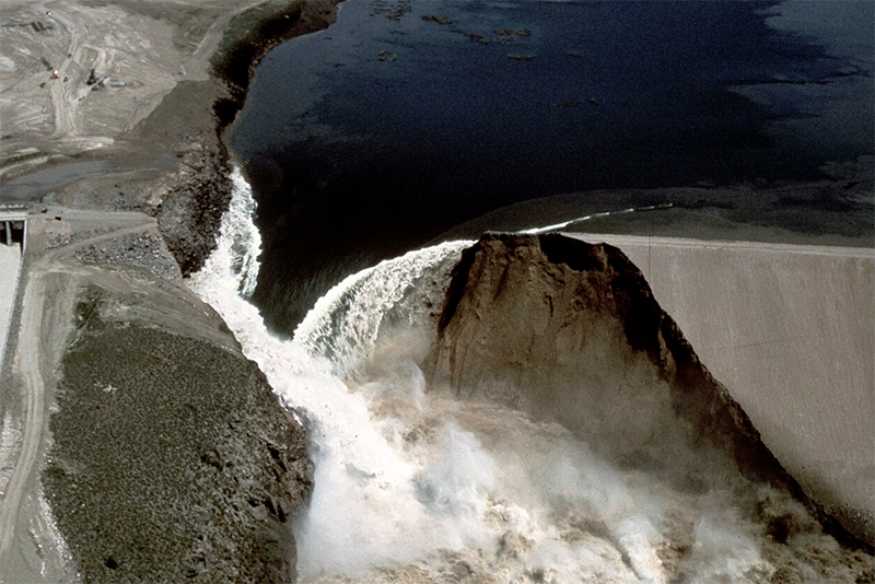
apreciablemente. Éste es el caso de una onda de inundación causada por la rotura de una presa.
Normalmente, la onda de inundación producida por la ruptura de una presa
de tierra dura aproximadamente 3 horas, lo cual la hace
un candidato seguro para una fuerte difusión de la onda.
Estas ondas de inundación (Fig. 4) tienden a caer en la categoría de ondas mixtas o, como mínimo, ser una onda de difusión fuertemente difusiva, con una atenuación
A ≅ 0.3
(consulte la Tabla 2, Línea 3a). Afortunadamente para todos, los casos de rotura de presas son raros.
9. MODELACIÓN DE ONDAS DE INUNDACIÓN Esta sección detalla formas de modelar ondas de inundación. Se busca responder a la pregunta: Ahora que elegí un tipo de onda, żCómo debo proceder? żQué herramienta real debería utilizar en una situación práctica? Esta sección se divide en tres partes: (1) ondas cinemáticas, (2) ondas difusivas, y (3) ondas mixtas. Las ondas dinámicas clásicas de Lagrange (véase la Sección 6) quedan fuera del alcance de esta sección. Ondas cinemáticas
El modelado de ondas cinemáticas se puede realizar de dos maneras. La primera es
darse cuenta de que una onda cinemática verdadera no se atenúa; por lo tanto,
la difusión está fuera de discusión.
La simplicidad de la celeridad de Seddon es notable, ya que proporciona una herramienta
inmediata para evaluar el movimiento de las inundaciones con un mínimo de esfuerzo.
La segunda forma de modelar ondas cinemáticas es utilizar un modelo numérico, varios de los cuales existen en diferentes formas, en la literatura. Estos modelos, sin embargo, adolecen del siguiente enigma: Cómo modelar numéricamente una onda cinemática sin introducir una cierta cantidad de difusión numérica asociada con el tamańo finito de la malla? [Téngase en cuenta que se supone que una onda cinemática propiamente dicha no tiene difusión; Ver Sección 4]. La difusión en cuestión no está controlada; su existencia puede confirmarse ejecutando el modelo para dos resoluciones de cuadrícula diferentes. Este ejercicio dará como resultado invariablemente dos respuestas diferentes, lo que plantea la pregunta de cuál es la solución correcta (Ponce, 1986). No parece haber salida a esta dificultad. En este punto, lo mejor que se puede afirmar es que, para una resolución de cuadrícula suficientemente fina, la difusión numérica debería reducirse hasta donde pueda no ser de gran importancia en una aplicación práctica determinada. Ondas difusivas A diferencia de las ondas cinemáticas, que se rigen por una ecuación diferencial de primer orden, la cual describe únicamente convección, las ondas de difusión se rigen por una ecuación de segundo orden, la cual describe convección y difusión. Hayami (1951) fue pionero en el desarrollo de la teoría de las ondas de difusión al combinar las ecuaciones de continuidad y movimiento, excluyendo los términos de inercia (Tabla 1, Línea 2), en una ecuación de convección-difusión de segundo orden. Esta metodología ha sido ampliamente referida en la literatura como la analogía de difusión de Hayami (Ponce, 2014a). . En el modelado de ondas de inundación, la solución numérica de la ecuación de convección-difusión de segundo orden proporciona una solución de onda difusiva.
Cunge (1969)
desarrolló una alternativa conveniente y práctica al
enfoque de Hayami, resolviendo numéricamente la ecuación de onda
cinemática de primer orden, al mismo tiempo relacionando
la cantidad de difusión numérica producida por el tamańo finito de la
malla con la difusión física real de la ecuación de convección-difusión
de Hayami. Cunge observó que su metodología de enrutamiento
de inundaciones se parecía al método clásico de Muskingum (1938),
citado por Chow (1959).
La característica reconocida de independencia de la malla
diferencia el método Muskingum-Cunge de las soluciones numéricas existentes de ondas
cinemáticas, las cuales sufren de dependencia del tamaño la malla.
Dado que la solución de la ecuación de la onda de difusión contiene, es decir,
abarca la solución de la ecuación de la onda cinemática, el procedimiento de
Cunge reemplaza tanto la solución de segundo orden de
Hayami como la solución de primer orden de la onda cinemática convencional, la cual es
dependiente de la malla. Por lo tanto, el método
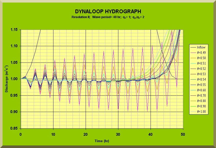
Ondas mixtas Las ondas mixtas comprenden todos los términos de las ecuaciones que rigen la continuidad y el movimiento del agua, es decir, las ecuaciones de St. Venant (Tabla 1, Línea 3). La inclusión de los términos de inercia es ciertamente contundente, pero no está exenta de condiciones. La onda resultante es dinámica, característicamente de segundo orden, por lo que presenta dos ondas componentes, que viajan en diferentes direcciones, una aguas arriba y otra aguas abajo en flujo subcrítico, y en la misma dirección (aguas abajo) en flujo supercrítico. La existencia de dos soluciones obstaculiza el propósito declarado del enrutamiento de inundaciones, que aparentemente es calcular la propagación de la onda primaria, es decir, específicamente la que viaja aguas abajo. Otro obstáculo importante es que la solución numérica de las ecuaciones completas de St. Venant representa un aumento de un orden de magnitud en la complejidad en la formulación y el rendimiento real del esquema numérico elegido para modelar las ecuaciones completas. Un esquema que parece ser ampliamente favorecido es el esquema de Preissmann (Ponce et al., 1978). Teóricamente, este esquema debería proporcionar una precisión de segundo orden, si sólo sus elementos (es decir, las derivadas temporal y espacial) están perfectamente centrados dentro del cuadro, con un factor de ponderación θ = 0,5. En la práctica, sin embargo, la ponderación central del esquema de Preissmann no funciona, pues conduce a fuertes inestabilidades numéricas, las que eventualmente lo hacen inoperable. Una forma conveniente de manejar este problema ha sido utilizar θ > 0,5, normalmente en el rango 0,55-0,60, con el fin de estabilizar el esquema, introduciendo una cierta cantidad de difusión numérica para controlar el cálculo. Valores mayores de θ, en el rango de 0,6 a 1,0, proporcionan cantidades cada vez mayores de difusión numérica, pero esto siempre se produce a expensas de una creciente falta de convergencia (Fig. 6). Por consiguiente, la metodología se degrada a primer orden, comprometiendo la ventaja original basada en el uso de un modelo completo de "onda dinámica", es decir, el modelo de onda mixta.
Otro problema importante en la solución numérica de las ecuaciones de St. Venant es que el modelo requiere
una condición de frontera aguas abajo para operar. Este hecho fue identificado tempranamente por
Abbott (1976): Extract, Page 276, como una verdadera limitación, aunque los defensores posteriores
de la metodología aparentemente no prestaron la debida atención a esta deficiencia. Por naturaleza,
el método genera curvas de gasto en bucle (léase histéresis) en puntos computacionales internos, lo que obliga a
especificar también una clasificación en bucle en la frontera aguas abajo. Claramente, este último requisito
equivale a "conocer la solución de antemano".
Seńalamos que los comentarios de esta subsección excluyen explícitamente el software
del gobierno de EE. UU., referido como Sistema de Análisis de Ríos del Cuerpo de Ingenieros
del Ejército de EE. UU., ampliamente conocido como HEC-RAS
En resumen, a estas alturas debe ser evidente que la onda mixta no es
lo que sus usuarios tenían en mente originalmente. Se ha demostrado en forma fehaciente que la onda mixta está
plagada de dificultades, la menor de ellas es saber si dicha onda está ahí o no para que
podamos calcularla.
10. ANÁLISIS Y CONCLUSIONES
Hemos analizado las propiedades de celeridad y atenuación de cuatro tipos de ondas
de aguas poco profundas actualmente utilizadas en ingeniería hidráulica: (1) cinemáticas,
(2) difusivas, (3) mixtas, y (4) dinámicas. Las ondas cinemáticas
son masivas (léase "grandes") y de hecho no difusivas.
Hemos tratado de responder a la pregunta de si la onda mixta es generalmente demasiado difusiva
para ser considerada una onda de inundación práctica. La respuesta es ˇSí! En la gran
mayoría de los casos, es posible que las ondas mixtas no estén ahí para que las
calculemos. Su típico tamańo mediano les obliga a atenuarse muy rápidamente, y su
masa se une eventualmente a la onda cinemática o difusiva subyacente,
la cual continúa creciendo tanto en tamańo como en permanencia a medida que se propaga aguas abajo.
Téngase en cuenta que sólo en el caso extremadamente inusual de una onda de inundación
que resulte de la rotura de una presa podríamos enfrentarnos al caso de una onda mixta.
Una onda de inundación que rompe una presa es característicamente repentina, preparada
por la Naturaleza para constituir una onda mixta, un tipo inusual de onda de
inundación [La experiencia de la falla de la presa de Teton (Fig. 4) es un
ejemplo de ello]. Los profesionales encargados de pronosticar o pronosticar retrospectivamente
una ola de inundación tras la rotura de una presa estarían interesados en
tener esto en cuenta. Para todas las demás aplicaciones de enrutamiento de
ondas de inundaciones, las ondas cinemáticas y difusivas deben hacer el trabajo de manera directa y precisa.
En particular, dado que una onda de difusión en realidad calculará la difusión, incluido el caso de
difusión cero, se deduce que la solución de una onda de difusión abarca la solución de una onda cinemática.
Por lo tanto, la onda de difusión se postula como la onda de inundación recomendada, es decir,
el tipo de onda generalmente indicada para su uso en aplicaciones prácticas de enrutamiento, y otras aplicaciones en
análisis y diseńo.
11. PALABRAS FINALES
En general, las ondas cinemáticas-dinámicas mixtas, aquí denominadas simplemente "ondas mixtas",
y que en otros lugares se han denominado ampliamente, postulamos aquÍ, de manera inexacta, "ondas dinámicas",
de hecho no son lo suficientemente grandes ni lo suficientemente permanentes como para constituir
verdaderas ondas de inundación. Un nutrido conjunto de teoría y experiencia confirma
este hecho. Por otro lado, las ondas cinemáticas y sus primas cercanas, las ondas difusivas,
suelen presentar una gran masa y son característicamente no difusivas, es decir, no se atenúan,
o se atenúan sólo una cantidad muy pequeńa; por lo tanto, tienden a ser modelos
ideales de ondas de inundación. Dado que la solución numérica de una onda difusiva
generalmente comprende la de una onda cinemática, la onda difusiva puede considerarse
como la forma más apropiada de modelar ondas de inundación.
REFERENCIAS
Abbott, M. B. 1976. Computational hydraulics: A short pathology: Extract: Page 276. Journal of Hydraulic Research, Vol. 14, No. 4, 271-285.
Chow, V. T. 1959. Open-channel hydraulics. McGraw-Hill, New York, NY.
Cunge, J. A. 1969. On the
Subject of a Flood Propagation Computation Method (Muskingum Method).
Journal of Hydraulic Research, 7(2), 205-230.
Fread, D. L. 1985. "Channel Routing," in Hydrological Forecasting,
M. G. Anderson y T. P. Burt, eds., Wiley, New York.
Hayami, I. 1951.
On the propagation of flood waves. Bulletin, Disaster Prevention Research Institute,
No. 1, Diciembre.
HEC-RAS. Hydrologic Engineering Center River Analysis System,
U.S. Army Corps of Engineers, Davis, California. Wikipedia citation (consultada
el 15 de mayo de 2024).
Lagrange, J. L. de. 1788. Mécanique analytique, Paris, part 2, section II, article 2, 192.
Lighthill, M. J. and G. B. Whitham. 1955.
On kinematic waves. I. Flood movement in long rivers.
Proceedings,
McCarthy, G.T. 1938. "The Unit Hydrograph and Flood Routing,"
unpublished manuscript, presented at a Conference of the North Atlantic Division,
U.S. Army Corps of Engineers, June 24.
(Citado por el texto de V. T, Chow "Open-channel Hydraulics," página 607).
Natural Environment Research Council. 1975. Flood Studies Report,
Vol. III: Flood Routing Studies, Londres, Inglaterra.
Ponce, V. M. and D. B. Simons. 1977.
Shallow wave propagation in open channel flow.
Journal of Hydraulic Engineering, ASCE, 103(12), 1461-1476.
Ponce, V. M. and V. Yevjevich. 1978.
Muskingum-Cunge Method with Variable Parameters.
Journal of the Hydraulics Division, ASCE, 104(12), December, 1663-1667.
Ponce, V. M., H. Indlekofer, and D. B. Simons. 1978.
Convergence of four-point implicit water wave models.
Journal of the Hydraulics Division, ASCE, 104(7), July, 947-958.
Ponce, V. M. 1982.
Nature of wave
attenuation in open-channel flow. Journal of Hydraulic Engineering, ASCE, 108(HY12), February, 257-262.
Ponce, V. M. and D. Windingland. 1985.
Kinematic shock:
Sensitivity analysis. Journal of Hydraulic Engineering, ASCE, 111(4), April, 600-611.
Ponce, V. M. 1986.
Diffusion wave modeling of catchment dynamics.
Journal of Hydraulic Engineering, 112(8), August, 716-727.
Ponce, V. M. 1995.
Hydrologic and environmental impact of the Parana-Paraguay waterway on the Pantanal of Mato Grosso, Brazil.
https://ponce.sdsu.edu/hydrologic_and_environmental_impact_of_the_parana_paraguay_waterway.html
Ponce, V. M. 2014a.
Engineering Hydrology: Principles and Practices.
Texto en línea.
Ponce, V. M. 2014b.
Fundamentals of Open-channel Hydraulics.
Texto en línea.
Ponce, V. M. 2024.
La onda cinemática desmitificada. Publicación en línea.
Seddon, J. A. 1900. River Hydraulics. Transactions, American Society of Civil Engineers, Vol. XLIII, 179-243, June; Extracto: páginas 218-223.
Taher-Shamsi, A., A. V. Shetty, y V. M. Ponce. 2003.
Embankment dam breaching: Geometry and peak outflow characteristics.
Documento en línea. En Español:
Wylie, C. R. 1966. Advanced Engineering Mathematics, 3rd ed., McGraw-Hill Book Co., Nueva York.
| ||||||||||||||||||||||||||||||||||||||||||||||||||||||||||||||||||||||||||||||||||||||||||||||||||||||||||||||||||||||||||||||||||||||||||||||||||